Regression

During the previous lessons, we learned that classification is predictic a label or a class for an entity. It was useful for predictic whether and image contains a number 0, 1, 2, (…) or 9. Regression is used for making predictions on a continuous-valued attribute such as price.

At this point, it is fair to warn that some of the terminology can be slightly misleading. For example, there is an algorithm called 'logistic regression' that is usually used for classification - not for regression. Thus, a regression model can be used for solving either regression or category problems.

Another source of confusion can be the word 'linear' in linear regression. The model itself is linear, single features can be polynomial.

• During this lesson, we will focus on regression models that are being used for performing regression analysis. We are interested in predicting a value of e.g. price, height, width or similar - NOT a category.
• During this lesson, we will focus on linear regression analysis using linear features.

Univariate Linear Regression

| Hours studied (x) | Point on Exam (y) | | ----------------- | ----------------- | | 17 | 188 | | 11 | 108 | | 6.5 | 98 | | 4.5 | 39 | | … | … |

On this artificial dataset, there is only one variable (also known as predictor): hours studied. We have 100 samples, consisting of hours studied and exam scores. If we were to plot the data on a graph, it would look like this:

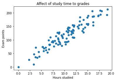
Remember that the data is completely artificial. We would now want to fit a straigh line right in the middle of the 'swarm' of samples. The line will be:

$ y = mx + b $

In the equation,

• m is the slope (in machine learning, it is a weight, also known as a coefficient)
• b is the bias term (where there line cuts y-axis)
• x is the variable (hours studied)
• y is the output variable (exam points)

When we get the values for m and b, we can predict how new students will score on the exam.

predicted_exam_points = slope * hours_studied + bias

Clearly, there is some noise in the dataset. Otherwise the features would form a completely straight line. This means that our model will never be fully accurate. Try for yourself: draw a straigh line into the graph so that it doesn't miss a single data point.

Normal Equation

But how would we get the values for bias and slope? We could use the normal equation to compute the weights (also known as coefficients). The equation will minimize the squared errors (the distance between the actual y-values and the line.) This is not a math course, so don't panic about the equation. We will just implement it. The equation is:

$ \theta = (X^T \cdot X)^{-1} \cdot X^T \cdot y $

In Matlab/Octave, the implementation would be:

pinv(X' * X) * X' * y

You could write the same in Python using linear algebra libraries, such as numpy, and it could look like this:

from numpy.linalg import inv

theta = inv(X.T @ X) @ X.T @ y

Bias term

The code above will only work if you add a bias term into your feature vector (X). A bias term is a constant 1 and it is added as a first column in your X feature matrix. See the table below.

| Column 0 of X (Bias term) | Column 1 of X (Study hours) | | ------------------------- | --------------------------- | | 1 | 8.77374662 | | 1 | 14.11851541 | | 1 | 6.95937414 | | 1 | 6.66081627 | | … | … |

Theta only has as many elements as you have features. We have two: the bias term and the hours studied. Theta is shown below in a table:

| Element 0 of Theta | Element 1 of Theta | | ------------------ | ------------------ | | 6.670141113817763 | 10.684098252285354 |

The prediction (y) will be computed using a dot product between the matrix X and vector theta:

$ y = \theta0x0 + \theta1x1 $

In practice, the first four rows:

| theta[0] * X[0] | + | theta[1] * X[1] | = | Exam score | | --------------------- | ---- | -------------------------------- | ---- | ------------ | | 1 * 6.670141113817763 | + | 10.684098252285354 * 8.77374662 | = | 100.40971201 | | 1 * 14.11851541 | + | 10.684098252285354 * 14.11851541 | = | 157.51374692 | | 1 * 6.95937414 | + | 10.684098252285354 * 6.95937414 | = | 132.97034773 | | 1 * 6.66081627 | + | 10.684098252285354 * 6.66081627 | = | 81.02477815 | | … | | … | | … |

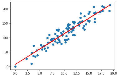
Below is the graph with the predicted y.

Normal Equation in Sci-Kit Learn

Why make things complicated when you can use an existing library? Let's import LinearRegression from sklearn and let it do all the heavy lifting for us. It even adds the bias term for us.

from sklearn.linear_model import LinearRegression

model = LinearRegression()
model.fit(X, y)

print(f"The slope is: {model.coef_[0]}")
print(f"The bias is: {model.intercept_}")

In this case, the output would be:

The slope is: 10.684098252285354
The bias is: 6.670141113817763

Now we could use these numbers for predicting new exam scores based on study hours.

hours_studied = 12

predicted_exam_points = slope * hours_studied + bias

print(f"Predicted scoring: {round(predicted_exam_points, 0)}/{round(max(y), 0)}")

In this case, the output would be:

Predicted scoring: 135.0/213.0

So far, we have built a model that predicts the exam points of students, but we have very limited tools for examining the accuracy of the model. In real-life example, we would've done the same as in k-NN example: take a portion of the dataset and use that for checking the performance of the model. We will do this later in this course. For now, focus on understanding linear regression without worrying about its accuracy.

Multivariate Linear Regression

It would be highly limiting in all prediction would compute the weights for a single feature with a single output value. What if we had more data than just 'hours studied'? Maybe we know a lot more, such as 'average hours slept' or 'grade of the previous course'. If the new input data correlates with the value we are trying to predict, then surely more features would increase the accuracy - at least to some limit?

As it happens, we can add more features the the feature matrix X. If we have n amount of features in the X, we will simply calculate the dot product of those:

$ y = \theta0x0 + \theta1x1 + \theta2x2 … \thetanxn $

For each feature in X, we will compute a weight. Weights are also known as coefficients. We will also compute a weight for the bias term, which will be added to be the 0th place in the X. Thus, the amount of weights in theta (symbol: θ) will have the same dimensionality as the input space. If you have 10 features, you will end up having 11 weights (one for each feature plus one for the bias term).

NOTE! In some libraries, the bias is kept separate from the weights. For example, Sci-Kit Learn's Linear Regression stores the coefficients (weights) and the intercept (bias) in separate variables.

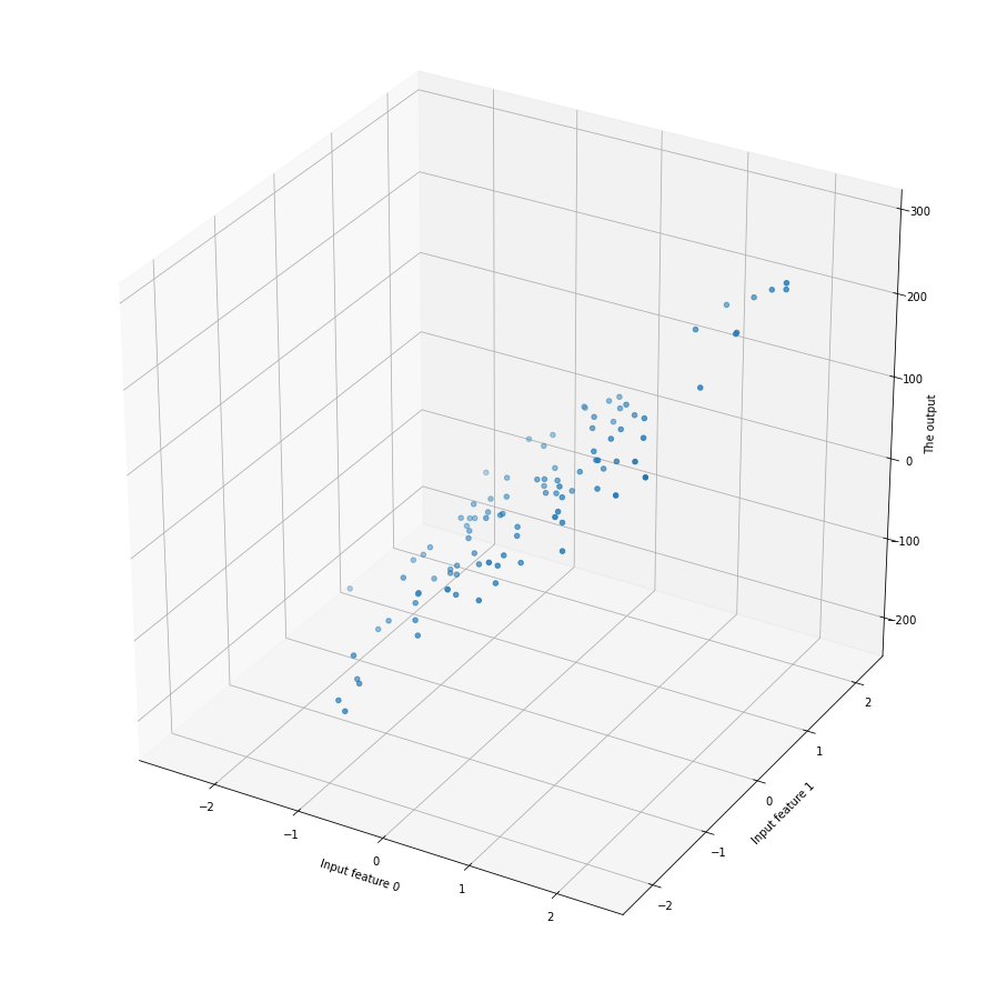
Above you can see a visualization of an artificial dataset that has 2 features. If you would plot the prediction into the graph, it would be a plane. Visualizing more than 2-dimensional datasets in a single graph is not practical; often you will see each feature plotted separately against the output (y).

Limitations of Normal Equation

def run_normal_equation_n_feats(n_features, n_samples):
    # Create ranomized dataset
    X, y = datasets.make_regression(n_samples=n_samples, n_features=n_features, noise=15)

    # Add the bias term to X
    bias = np.ones(((n_samples,1)))
    X = np.c_[bias, X]

    # Compute the theta
    theta = inv(X.T @ X) @ X.T @ y

# Set m*n for X
feature_counts = [10**2, 10**3, 10**4]
sample_count = 10**4

# Initialize a list for times
times = []

for n in feature_counts:
    start = datetime.datetime.now()

    run_normal_equation_n_feats(n, sample_count)

    deltatime = (datetime.datetime.now() - start).total_seconds()

    times.append(deltatime)

Running the code above demonstrated how the computational time increases when the dimensionality of X increases.

# X with 10^2, 10^3 and 10^4 features
# X containing 10000 samples
# Time in seconds
[0.070227, 0.836989, 45.762016]

# X containing 20000 samples
[0.12601, 1.603985, 70.381015]

Normal equation is fast, assuming that there are less than about 10^4 features and not too many samples for your computer's memory. The limitations of normal equation is that, whilst it computes everything at once, it is not unrealistic in situations where you have large number of features. If this is the case, you must use some other algorithm that can compute the weights iteratively - either just one training example at a time or in small batches. One suitable algorithm would be Stochastic Gradient Descent. You will learn to implement SGD during this course!