Feature Scaling

When we trained fitted k-NN classifier to MNIST data, we got surprisingly good results without performing any sort of data cleaning or feature handling. This is usually not the case; especially with an algorithm such as k-NN that simply calculates the Euclidean distance in n-dimensions. With MNIST, we had 64-d (8x8 pixels) feature vector, where each feature was a pixel intensity on scale of 0 to 16. All the features shared the same scale so Euclidean distance makes sense. What about the BackBlaze dataset? It has multiple features, of which two were:

• capacity_bytes which has a max() of 16,000,900,661,248
• smart11raw which has a max() of 12,201

What might happen if these two features (disk capacity in bytes and recalibration retry count) would be compared to each other using Euclidean distance? Imagine that you would compare these three drives:

• DISK A: 16 TB drive with smart11raw of 10k
• DISK B: 8 TB drive with smart11raw of 10k
• DISK C: 4 TB drive with smart11raw of 60k (alarmingly, strangely high value!)

The k-NN classifier predicts the class based on Euclidean distance. Assuming that the C drive is supposed to be the anomaly; the drive with failure 0, we would want to see that the Euclidean distance grows if the value gets abnormally large - as it did with the Disk C. Let's perform some calculations! (Note! We are assuming that a 1 TB is exactly 10^12 bytes. It is not in real life.)

from scipy.spatial.distance import euclidean
import itertools 

disks = {"A": [16*10**12, 10000], 
         "B": [ 8*10**12, 10000], 
         "C": [ 4*10**12, 60000]}

y = {"A": 0, "B": 0, "C": 1 }

for left, right in itertools.combinations(disks, 2):
    dist = euclidean(disks[left], disks[right])
    print(f"{left}<->{right}: {dist}")

Output in table form:

| From | To | Euclidean Distance | | ---- | ---- | ------------------ | | A | B | 8000000000000.0 | | A | C | 12000000000000.0 | | B | C | 4000000000000.0 |

Notice that the distance between any two disks is the same as the capacity. One dimension is in trillion, another is in thousands. The smart_11_raw of disk C would have to kick up to 2-3 million before it would even affect the Euclidean distance beyond the decimal point.

It surely would make sense that different variables would share a same unit. You wouldn't compare distances with feet and meters being mixed up either, would you?

Normalizing to 0…1

One way to scale your feature would be to normalize the values between 0 and 1. The

$ normalizedi = \frac {xi - x{min}}{x{max} - x_{min}} $

import numpy as np

# Create an array
x = np.array([ -2.05, -1.1, 0, 1.05, 2.01])

# Normalize min-max to 0-1
x_norm = (x - x.min()) / (x.max() - x.min())

print(x_norm.round(2))

The output on console:

[0.   0.23 0.5  0.76 1.  ]

Tip: there are cases where x.min() or x.max() can be replaced with a known value, if the feature has a known maximum. A prime example is 8-bit image data, where you know that the value range is between 0 and 255. In this case, the normalization would be as simple as x_norm = x / 255. (If the minimum is zero, there is no point subtracting it from anything.)

Normalizing to a…b

The code below showcases how to scale the normalized x_norm to any given range between low and high.

# Set the limits
low = -1.0
high = 1.0

# Perform scaling
x_normscaled = x_norm * (high - low) + low
print(x_normscaled.round(2))

The output on console:

[-1.   -0.53  0.01  0.53  1.  ]

Tip: This can also be used for rescaling the x_norm back to its original range. For this, you would set low = x.min() and high = x.max()

The same results can be achieved by using sci-kit learns MinMaxScaler.

from sklearn.preprocessing import MinMaxScaler

# Construct the object
mms = MinMaxScaler(feature_range=(0,1))

# Perform fit and transform 
x_norm = mms.fit_transform(x.reshape(-1,1))

# Perform inverse transform
x_reverted = mms.inverse_transform(x_norm).flatten()

The result of normalization gets changed slightly if minimum or maximum values change. This makes is somewhat vulnerable to outliers. Outliers are data points that do not fit to the distribution of other points in the population. These anomalies might be naturally existing, or they might by some mistakes in data collection. Having that said, outliers should be cleaned from the dataset. There is no normalization methods that would magickly make all outliers disappear.

Let's try normalizing a feature from the BackBlaze dataset. Let's choose the familiar smart9raw: the Power-One Hours.

# Other imports hidden since you are already familiar with pd, np and sns
from sklearn.preprocessing import MinMaxScaler

# Load BackBlaze data
data = pd.read_csv("02-data/2020-01-01.csv", usecols=["model", "smart_9_raw"])

# Min-Max Normalize the capacity
mms = MinMaxScaler()
data["min_max_norm"] = mms.fit_transform(data.smart_9_raw.values.reshape(-1, 1))

sns.distplot(data.min_max_norm, kde=False)

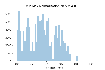
The last two rows of the DataFrame would look as follows:

| | model | smart9raw | minmaxnorm | | -----: | -------------------: | ----------: | ------------ | | 124953 | HGST HMS5C4040BLE640 | 24534.0 | 0.412912 | | 124954 | ST12000NM0007 | 2552.0 | 0.042951 |

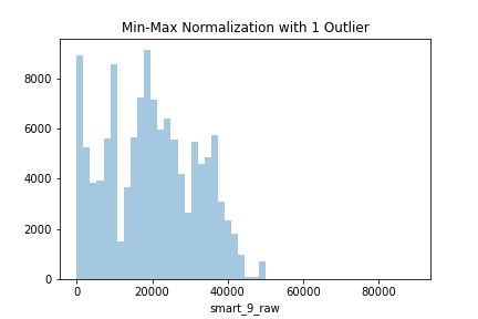
There are no outliers in the dataset, so this worked quite fine. Wonder what happens if we append an outlier to the dataset. The new disk added to the dataset is my FakeBrand and the model is MADEUPHDD_3000. The capacity is 12 terabytes, but the feature variable has been written in bytes. Thus, instead having the value 12 like other 12 terabytes drives in our dataset data ,

# Append the outlier to the DataFrame
data = data.append(pd.Series({"model": "MADE_UP_HDD_3000", 
                              "capacity": 12000138625024}), 
                               ignore_index=True)

# Normalize the data
data["capacity_normalized"] = mms.fit_transform(data.capacity.values.reshape(-1, 1))

# Visualize
sns.distplot(data.capacity_normalized, kde=False)

The last two rows of the dataset would look as follow:

| | model | smart9raw | minmaxnorm | | -----: | ---------------: | ----------: | -----------: | | 124954 | ST12000NM0007 | 2552.0 | 0.028634 | | 124955 | MADEUPHDD_3000 | 89125.5 | 1.000000 |

Notice how all values (except the outlier) got pushed closer to the 0, since a new maximum value was introduced to the dataset. This is an extreme case, of course, but it demonstrates how outliers affect the min-max normalization.

Z-score standardization

Z-score standardization (also known as standard score) by far the most common method of standardizing features.

During this course, we have aggregated features using methods such as sum(), max(), min() and mean(). If we add another tool into the mix , std(), we have all the ingredients needed for standard scaling. The std() stands for standard deviation. If you don't recall what standard deviation is, you might want to recap your math or statistics books. In short, it is a value that describes a typical distance from mean. The higher the value, the more spread out your data is.

The previous method normalized the values from one range to another, but the relative distances remained the same. Z-score takes another approach. It translates the data so that the mean() will be zero and std() gets scaled to 1. The formula is:

$ zi = \frac{xi-x{mean}}{x{std}} $

# Create an array. Compute standard deviation and mean.
x = np.array([ -2.05, -1.1, 0, 1.05, 2.01])
s = x.std()
u = x.mean()

# Perform standard scaling
z = (x - u) / s

print(z)

Output is:

[-1.39865583 -0.7447567   0.01238967  0.73512029  1.39590257]

The same can be achieved using the StandardScaler in scikit learn.

# Instantiate, fit and transform
from sklearn.preprocessing import StandardScaler
ss = StandardScaler()

z = ss.fit_transform(x.reshape(-1, 1))

print(z.flatten)

When using the StandarScaler, the object will hold the values for std and mean. These variables can be accessed using ss.mean_ and ss.scale_. The operation can be inversed by calling ss.inverse_transform(z) or by computing x_orig = z * s + u.

How would StandardScaler perform with the BackBlaze dataset that contains the artificial outlier? Let's try.

# Load BackBlaze data
data = pd.read_csv("02-data/2020-01-01.csv", usecols=["model", "smart_9_raw"])

# Perform StandardScaling
ss = StandardScaler()
data["sscale"] = ss.fit_transform(data.smart_9_raw.values.reshape(-1, 1))

plot = sns.distplot(data.sscale, kde=False, hist_kws={'range': (-3.0, 3.0)})

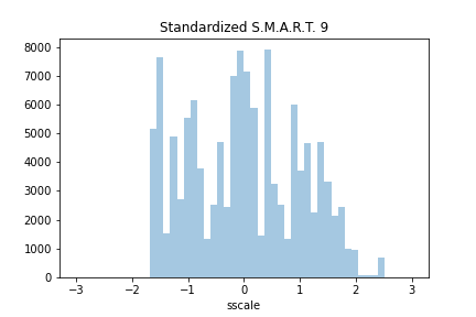
The last two rows of the dataset are:

| | model | smart9raw | sscale | | -----: | -------------------: | ----------: | --------- | | 124953 | HGST HMS5C4040BLE640 | 24534.0 | 0.392948 | | 124954 | ST12000NM0007 | 2552.0 | -1.455936 |

If we append the fake HDD to the dataset, the effect on the histogram is not even noticeable.

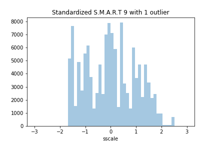
The last two rows of the dataset, after appending the fake HDD, are as follow:

| | model | smart9raw | sscale | | -----: | ---------------: | ----------: | --------- | | 124954 | ST12000NM0007 | 2552.0 | -1.455791 | | 124955 | MADEUPHDD_3000 | 89125.5 | 5.824858 |

Conclusion

So, which is better? It depends on your dataset and on your model. You might need to compare multiple scalers when you are trying to improve the performance of a given model.

Also, these there are a lot of other scalers available. Scikit Learn provides an example script for comparing various scalers visually. Take a look.

Open up the Jupyter Notebook and see how all you've learned enables you to predict whether a passenger survives Titanic or not.