Dimensionality Reduction
This lesson is a brief overview of an unsupervised learning technique called dimensionality reduction. The algorithm we will be using is Principal Component Analysis (PCA). In short, PCA does its best in explaining the dominant causes of the variation in our training set.
There might be multiple reasons to perform dimensionality reduction, including:
- Fight the curse of dimensionality. As mentioned before, high-dimensional non-zero matrices are sparse.
- Compress data. This will reduce the file size and also speed up the training of the machine learning algorithm.
- Help in visualization. Since understanding more than 3-dimensional plots is troublesome, you might need to reduce the dimensionality of your dataset from n_dimensions to 3 in order to plot the data.
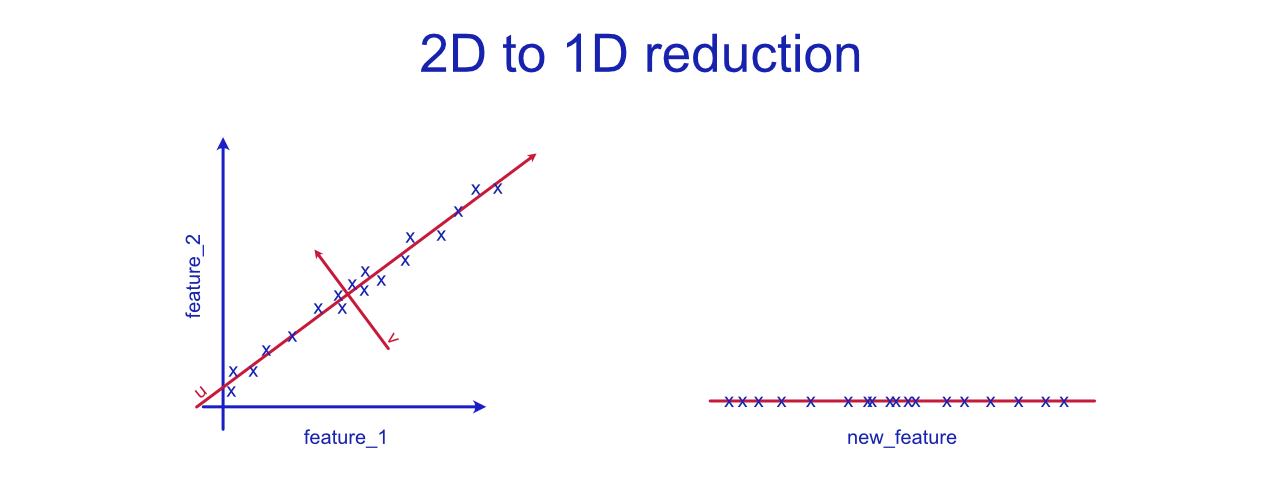
Above you can see a graph that visualizes how two features could be compressed into feature. Let's imagine that the original features are fermentation_time and dough_tastiness. These two variables seem to be highly correlated and the correlation seems linear. The collinearity between variables can hurt the performance of various machine learning algorithms. In this simple example, we could fix this by simply removing one of the features, but wen the dimensionality is huge and the contents of various features is less obvious, manually omitting features is not a reasonable thing to do. PCA algorithm would try to fit a straight line to the dataset that explains most of the variance in the data. This is the first principal component, also known as eigenvector, is u. The end line is close to what linear regression would plot, but notice that it is not the same thing. We have no y here. The second principal component or eigenvector, v , would be orthogonal (at 90 degrees angle) to the first principal component. These two components, u and v, form a new uv-coordinate system. Instead of simply re-basing our coordinate system, we want to reduce the dimensionality from 2-d to 1-d. Thus, we will only keep the more-descriptive eigenvector, u.
On the right side of the graph, we have the newly created feature (the "u" eigenvector). In this case, we could call it dough_maturity. The new feature does explain most of the variance, but there is still some projection error. This error is created by the distances between actual samples and the PCA vector. The greater the variance (in v direction), the more data we will lose. In the best case scenario, we will simply lose some unnecessary noise.
If you have ever done photography, you know that the photograph is a 2D representation of the 3-dimensional object. If you are photographing a fairly flat object, such as a leaf, the photograph will do justice to the actual dimensions of the object. For non-flat objects, you have to choose which silhouette you will keep.
In unsupervised learning, projecting from 3D to 2D would mean fitting a plane. For dimensions larger than 3, it will be a hyperplane.
Iris Dataset Example

The image above is from Scikit Learn's example, in which the four features of Iris dataset have been reduced to 3-d. Check the code at Scikit Learn website. With the 2-dimensional example, it was fairly easy to find a name for the newly created feature. How would you call these three features? They are the three eigenvectors that describe the variance the best, but… what are they? Let's investigate.
After fitting and transforming the data, let's create a Pandas DataFrame that we can examine:
# Create the DataFrame
df = pd.DataFrame(pca.components_, columns=iris.feature_names)

# Add new column
df["Explained Variance %"] = pca.explained_variance_ratio_

# Round to 2 decimal places and translate.
df.round(2).abs().T
Output:
| RAW FEATURES | PC-1 | PC-2 | PC-3 | | -----------------------: | -------: | -------: | -------- | | sepal length (cm) | 0.36 | 0.66 | -0.58 | | sepal width (cm) | -0.08 | 0.73 | 0.60 | | petal length (cm) | 0.86 | -0.17 | 0.08 | | petal width (cm) | 0.36 | -0.08 | 0.55 | | Explained Variance % | 0.92 | 0.05 | 0.02 |
For now, ignore other values than the explained variance. The first principal component (PC-1) explains 92% of the variance in the whole dataset. If seems that the PC-1 contains the "rough guidelines" for classifying the Iris species. If we were to rotate the 3D graph slightly, it would become clear how important the PC-1 is for classification. Look at the graph below.

The complete explained ratio can be calculated as sum(pca.explained_variance_ratio_) and in this case, it is ~0.995 (99.5 %). With n_components=4, the total explained variance ratio is 1.00 (100 %). This applies to any dataset where n_components=n_features, since we are simply re-basing the coordinate system. Anything below 100 % means that we are losing some variance.
So, how did we arrive to these numbers? The full mathematical explanation is beyond the scope of this course, but if we use the covariance method, the steps would be as follows:
Covariance Matrix
The covariance matrix of our features is calculated. If you want to do this yourself, you can call np.cov(X.T). The output is always a square matrix where the diagonal values are 1 (when rounded), since they represent the covariance of the element with itself. You can also access the covariance matrix by calling pca.get_covariance() after fitting the data.
The values in the covariance matrix indicate the covariance between each pair of elements. Below is a heatmap visualization.

Eigenvectors
The next step is to decompose the covariance matrix using eigen decomposition. "Eigen" is a German word meaning 'self'. Eigenvalues and eigenvectors are the "self-components" of a given matrix that explain what the matrix 'does.' You can compute these using NumPy:
eigenvalues, eigenvectors = np.linalg.eig(covariance_matrix)

print(eigenvectors.round(2))

# OUTPUT:
#[[ 0.36 -0.66 -0.58  0.32]
# [-0.08 -0.73  0.6  -0.32]
# [ 0.86  0.17  0.08 -0.48]
# [ 0.36  0.08  0.55  0.75]]
Notice that the eigenvectors are the exact same values as in the table above. So PC-1 is eigenvectors[:, 0] with values [ 0.36, -0.08, 0.86, 0.36]. The fourth column is the PC-4 that we decided not to use (by choosing n_components=3)
eigenvector_from_sciki = pca.components_[0].round(2)
eigenvector_from_numpy = eigenvectors.T[0].round(2)

eigenvector_from_sklea == eigenvector_from_numpy

# OUTPUT
# [True, True, True, True]
Eigenvalues
# Remember, we got both eigenvectors and eigenvalues by calling
eigenvalues, eigenvectors = np.linalg.eig(covariance_matrix)

# The eigenvalues hold values:
eigenvalues.round(2)
# [4.23, 0.24, 0.08, 0.02]
If you need to access the same numbers using Scikit Learn, you can call pca.explained_variance_. Although, it will only return as many values are you chose when constructing the PCA. In our case, this number was n_components=3.
pca.explained_variance_.round(2)
# [4.23, 0.24, 0.08]
Notice: The pca.explained_variance_ is different from pca.explained_variance_ratio_. The latter can be calculated using eigenvalues. For the first principal component PC-1, the ratio would be eigenvalues[0] / sum(eigenvalues) that equals ~92 %. This is the same value as in the table above.
Translate the values
We can use the PCA to perform the dimensionality reduction by calling the fit and transform (or both at the same time by calling fit_transform). This is expected behavior, but let's test it anyways:
# Use the Scikit Learn PCA
X_pca = PCA(n_components=3).fit_transform(X)

# The rounded output is:
X_pca[0].round(2)
The output of this script is the first sample in our database described using the 3 synthetic features. Values are: [-2.68 0.32 -0.03]. The first flower in our database has -2.68 units of PC-1, 0.32 units of PC-2 and -0.03 units of PC-3. What are these components? Let's discuss that later.
If we want to reach the same numbers as Scikit Learn, we can use the knowledge we already have. We will need eigenvectors!
# Covariance Matrix
X_cov = np.cov(X.T)

# Get the eigenvectors. We don't need eigenvalues for this.
_, eigenvectors = np.linalg.eig(X_cov)

# Center the data so that mean is 0. PCA() also does this.
X_cent = X - np.mean(X, axis=0)

# The new features are the dot product of our X and eigenvectors
X_pca_np = X_cent @ eigenvectors[:, :3]

# The rounded output is:
X_pca_np[0].round(2)
The output is:
[-2.68 -0.32 -0.03]
The absolute values match to those of PCA(), but the PC-2 feature has an opposite sign. Notice that this doesn't break anything. Imagine if you flip the North-South directions in a map. The map will be mirrored in vertical direction, but the relative distances remain the same. The map would be highly non-conventional, but it wouldn't stop you from using it for finding a route from location A to B.
Extension Task: Feel free to investigate why the sign is flipped. If you check the source code of PCA class and its base class, you will notice that Scikit Learn uses SVD instead of calculating the covariance matrix. The get_covariance() method uses the components produced by SVD to compute the covariance matrix. Our approach required the covariance matrix to be created as a first step. Scikit Learn uses SVD since it is efficient with larger matrices.
The Importance of Standard Scaling
If you check the Scikit Learn's code, you will notice that they are not using standard scaling. The PCA doesn't apply it by default: check the documentation to confirm. You want to always scale the dataset to unit scale (so that the mean is 0, std is 1) before applying PCA.
Note: With Iris dataset, skipping this didn't cause major problems since all features share a real-life unit (centimeter) and are roughly similar in scale distributions, but even in this case, it did cause the sepal length to be seen as an overimportant feature.
Below is the same table as before, but this time with scaled features (using the Scikit Learn StandardScaler.)
| SCALED FEATURES | PC-1 | PC-2 | PC-3 | | -----------------------: | -------: | -------: | -------- | | sepal length (cm) | 0.52 | 0.38 | -0.72 | | sepal width (cm) | -0.27 | 0.92 | 0.24 | | petal length (cm) | 0.58 | 0.02 | 0.14 | | petal width (cm) | 0.56 | 0.07 | 0.63 | | Explained Variance % | 0.73 | 0.23 | 0.04 |
Notice that the explained variance for PC-1 has dropped to 73 %. This is due to the change of our unit. Prior to the scaling, the petal length feature contained the largest values, and since PC-1 has high correlation with petal length, the explained variation was exaggerated.
Remember that these PC-1, PC-2 and PC-3 features are synthetic, but they correlate with various existing plant features. Plotting only the PC-1 reveals how a classifier could perform on a single, most important component. Setosa (the bottommost label) is easy to classify. The other two species overlap, which would impact the accuracy of our classifier.

Adding the second component, PC-2, doesn't completely remove the overlap, but if we were to use polynomial features, we would definitely be able to (over)fit a line that separates the groups. (Remember: overfitting is problem, so we would either have to accept a slightly lacking accuracy or get new features. Maybe find some plants and get some new kind of measurements?)

If we were forced to name these synthetic features, how would would we do it? PC-1 has positive, fairly equal correlation with all measurements except sepal width. So, if a plant has large leaves but narrow sepals, it resembles virginica. Maybe we could call this petal_dominance_in_area. The components created using PCA doesn't necessarily fit the human intuition that well.
Conclusions
Dimensionality reduction is a range of techniques used for shrinking the feature space. Head to the Jupyter Notebook to find out how you can use PCA to reduce the nfeatures to ncomponents. A potential drop in features/components is from 4096 to 64. Even with this tiny amount of features, you can still render the image so that both you and a classifier algorithm can identify the people in X_train. Neural networks are the state of the art approach for face recognition and identification, but even this simple technique can reach surprisingly high accuracy with limited number of labels (=names/individuals).