Perceptron

The Perceptron algorithm was invented in 1950s and in consist of a single neuron with n inputs. It computes a weighted sum. The Perceptron has been implemented in Scikit Learn in linear_model.Perceptron.

The Sci-Kit documentation states that:

In fact, Perceptron() is equivalent to SGDClassifier(loss="perceptron", eta0=1, learning_rate="constant", penalty=None).

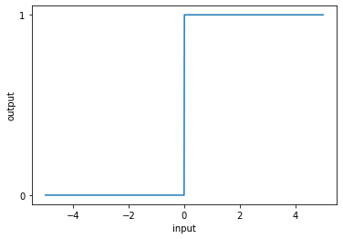
The perceptron is a linear algorithm and it has a linear activation function called step function or heaviside function. This activation function fires (meaning it outputs 1) only if the input is positive.

def step_function(x):
    return 1 if x >= 0 else 0

When plotting input values of range np.linspace(-5, 5, num=100), the graph looks like a stairstep:

The whole graph is illustrated below:

• X matrix is our input data

• …and it has m samples with n features.

• W are our weights for each n feature (including the bias)

• Σ is the sum

• …and the last element is our step function step.

Thus, the output (either 0 or 1) will be calculated as:

$ output = step(x0w0 + x1w1 + x2w2 \cdots wnwn) $

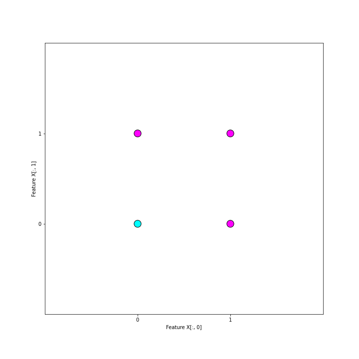
The dataset we will be using contains only four samples:

• x_1 = [0, 0]
• x_2 = [0, 1]
• x_3 = [1, 0]
• x_4 = [1, 1]
• Our y is [0, 1, 1, 1]. It follows logic feature[0] or feature[1].

Below you can see the scatterplot of our dataset:

The goal of our training is to adjust the weights so that the predictions match the ground-truth - just as with all the linear classifiers we've used before. The update rule is called perceptron learning rule or delta rule.

$ W{new} = W{old} + \alpha (\hat y - y)x_n $

• Notice that the ŷ - y is the error and it has only three potential values: [-1, 0, 1].
• If the prediction equals the ground truth, meaning that ŷ == y, the error is exactly zero, since 0 - 0 = 0and 1 - 1 = 0.
• If the error is 0, the right side of the formula will equal zero, since alpha * 0 * x is always zero.
• The alpha is a small scalar such as 0.01
• The x_n is any sample in our dataset X. [[0,0], [0,1], [1,0], [1,1]]

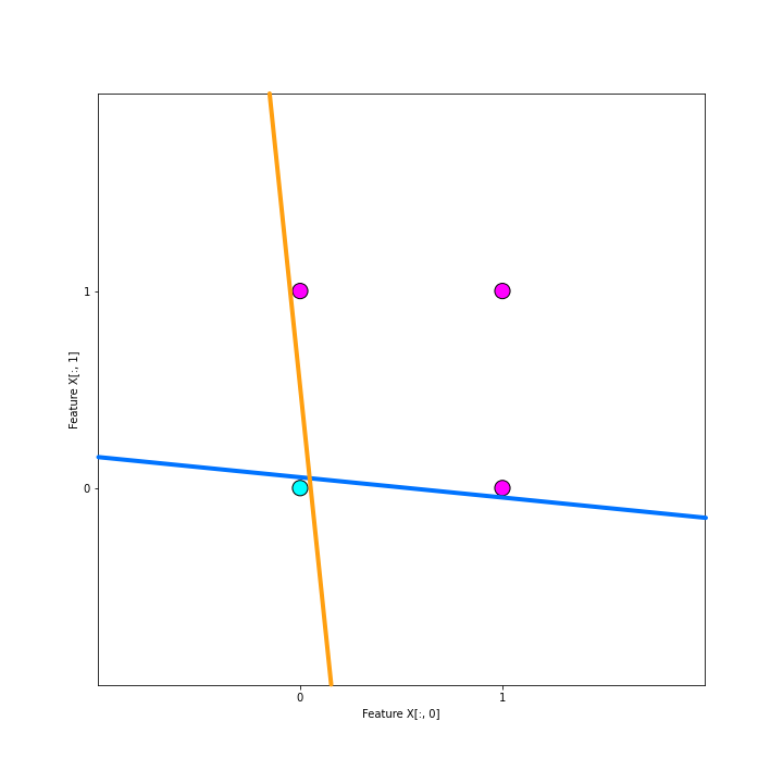
In the Jupyter Notebook section, you will see how we fit the model to the data iteration-by-iteration. In the end, we will end up with various decision boundaries, including the two in the graph below. The final decision line is guaranteed to get 100 % accuracy on a linearly separable set (such as our OR-problem), but the position of the decision boundary may vary. The two decision boundaries plotted below are nearly perpendicular - and they both are essentially "right" solutions!

Conclusions

Notice that both lines in the graph above produce total error of 0, meaning that no weights will be updated. This means that the algorithm has no way of improving the fitting any further.

Another limitation of perceptron is that it can only deal with linearly separable datasets, unless we swap out the cost function and the activation function, apply some calculus and add hidden layers to out network. This is what we will be doing in the next lessons.

It is fairly unlikely that you will ever end up using the vanilla perceptron algorithm in any real classification task. Having that said, understanding the single-layer perceptron helps us in understanding the multi-layer perceptron and other feed-forward multilayer neural networks (and thus deep neural networks).

HOMEWORK: Read the section "Perceptrons" in Chapter 1: Using neural nets to recognize handwritten digits of the online book Neural Networks and Deep Learning.