Optimization and Regularization

Let's continue from where we left. During the last Notebook exercise, we created a couple of cost functions. This time, we will be writing an algorithm from scratch called gradient descent. If we want to find the global minimum (the value that will minimize the cost), our cost needs to be a convex function.

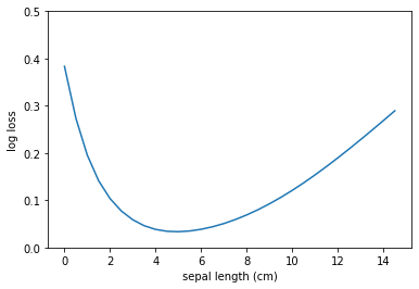
A strictly convex cost function will have a U-shape; the top part of this function is a convex set. If you choose two values and draw a line between those two points, the line will never leave the area. Read Wikipedia or a math book for more information.

The intuition behind gradient descent is simple. Your machine learning model is a tiny bee that has just landed inside a bowl. The bee wants to find the bottom of the bowl. The bee has been told that there is cake. Unfortunately, the bee is blind, so it cannot see where the global minimum is, but she has a good sense of balance. The bee has also been told that the bowl is large: the diameter might be anywhere between 2 to 20 meters. Walking downhill until arriving to the destination would take too much time; the bee is a slow walker, but can fly be pretty fast. Thus, the bee decides to fly! But how far? The bee takes a rough guess: the global minimum might be 1 meter away from its current position. The bee flaps its wings, rises to a safe flying height (directly up), flies about 1 meter to the direction of the global minimum and lands (directly down). Based on where the bee landed, it can draw some conclusions:

• The ground is flat. What a luck! The bee is as close as the global minimum as it can get (limited by the accuracy of her sense of balance).
• The spot where the bee landed is downhill.
  • If the slope is nearly as steep as before (similar angle), the 1 meter was a bit too optimistic guess. It would be a good option to continue flying to the same direction, but maybe 2 meters this time.
  • It the slope is less steep (lower angle), a good option would be fly another meter towards the same direction - or maybe even less than 1 meter.
  • If the slope is pointing to the opposite direction, the bee must have flown over the global minimum. It would be a good idea to turn around (180 degrees) and fly, say, only 50 centimeters this time.

By repeating the process above, the bee will eventually find the cake that is somewhere in the bottom of the bowl.

Defining Gradient

Our model doesn't have sense of balance like the bee. So, how to find the direction? We do this by computing the gradient. Definition of gradient according to Google Machine Learning Glossary is: "The vector of partial derivatives with respect to all of the independent variables. In machine learning, the gradient is the vector of partial derivatives of the model function. The gradient points in the direction of steepest ascent." A partial derivative is defined by the same source as: "A derivative in which all but one of the variables is considered a constant."

Remember that the selected cost function depends on whether you are building a regressor or a classifier. For regression problems, you will most likely be using some variation of squared loss such as Mean Squared Error. For classification problem, you will most likely use log loss (cross entropy) or hinge loss. The selected cost function needs to be suitable for the problem; if you cannot calculate the gradient, you cannot perform gradient descent. How you actually compute the gradient depends on your cost function.

Computing the Gradient of (halved) MSE

To compute the gradient numerically by iterating over the items in X and W, we need to compute the partial derivates for each weight individually. We could use pen and paper to formulate the derivation, but let's use the SymPy library, which is a module for performing symbolic mathematics in Python. Notice that the variables y, w0, w1... are never give any numerical values. Instead, they are symbols. The diff() function computes the derivate forms for our single-item cost function.

import sympy as sym

y, w0, w1, x0, x1 = sym.symbols('y, w0, w1, x0, x1')

cost = (y - (t0 * x0 + t1 * x1))**2 / 2

cost.diff(t0)
cost.diff(t1)

For the sample X[i], the W[0] (the intercept) and W[1] (the coefficient) would have their partial derivatives as:

$ partial0 = -x0(-w0 x0 - w1 x1 + y_i) $

$ partial1 = -x1 (-w0 x0 - w1 x1 + y_i) $

You may have noticed that the single-sample cost has been modified; we are dividing it by 2 (=halving it). The reasoning is simple: to keep the formula to compute the partial derivatives shorter. Try running the code above with and without the / 2. You will notice that adding the extra divisor makes the derivate formula one variable shorter. Let's put these formulas into use in Python:

# Empty list to hold the single-item partial derivatives
W_0_partials = []
W_1_partials = []

for i, x in enumerate(X):
    temp_0 = -x[0] * (-W[0] * x[0] - W[1] * x[1] + y[i])
    temp_1 = -x[1] * (-W[0] * x[0] - W[1] * x[1] + y[i])

    W_0_partials.append(temp_0)
    W_1_partials.append(temp_1)

As you can see, we are simply iterating over elements in X. Each element in X is x = X[i]. (Notice the case-sensitivity! capital X is the whole dataset, lower-case x is a single row.) Thus, the ground-truth for any xinside the loop is the y[i]

Now, to get the full cost, we need to compute the mean of each weight. This will give us the gradient of the (Halved) Mean Squared Error.

# Mean of partial derivatives
w_0_mean = sum(W_0_partials) / m
w_1_mean = sum(W_1_partials) / m

# Stack vertically to get the gradient
gradient = np.vstack((w_0_mean, w_1_mean))

In this bivariate case, the W would be of shape (2,1). Thus, also the gradient needs to be in the shape (2,1). The contents of this array could be, for example:

# Example output of print(gradient)
[[ -16.15126649]
 [-126.62975594]]

Currently, the code above is fixed for 2 features (incl. bias), having only 2 weights. How would you change it to fit n_features > 2? Feel free to try to implement this yourself.

Learning Rate

In the example case above, the values of the weight matrix W were W[0] = 0.5 and W[1] = 0.5. The absolute values in the gradient vector are huge compared to our weight values (such as 126.6 versus 0.5). If we use these values as a step size, imagine what will happen. Our "machine learning bee" will fly past the base of the bowl and continue some extra (hundred) meters to the wrong direction. The poor bee would never find the cake. Thus, if we want to take a small step towards global minimum, we need to multiply it with some tiny value, which is usually known as an alpha or as a learning rate. The optimum or correct value is a hyperparameter you tune when improving your model. By convention, negative powers of ten are used as a starting point, such as 1e-3 = 0.001. This value needs to be tweaked if learning is too slow or doesn't happen at all.

learning_rate = 1e-3
step = learning_rate * gradient

Now, the step-sizes will be one thousandth of the original:

# Example output of pring(step)
[[-0.01615127]
 [-0.12662976]]

Since the W and shape arrays share the same dimensions, we can simply perform element-wise subtraction to update the weights:

# Change the weights based on the step size
W -= step

Vectorized form

Looping is time-consuming and we should favor vectorized form of computation to take benefit of parallel computing. The vectorized form over n features is:

$ gradient = -\frac{1}{m}X^T (y - y_{hat}) $

This is also implemented in the Exercise Notebook in Python, so read through the Notebook with care.

Running a cell with %%timeit magic function displays the average runtime per cell over a few trials. Below, you can see the timings when run on a fairly powerful laptop computer:

%%timeit

# VECTORIZED
gradient_descent(X_train, y_train, W, vectorized=True)

# Output: 128 ms ± 991 µs per loop (mean ± std. dev. of 7 runs, 10 loops each)

By looping:

%%timeit

# NON-VECTORIZED (=LOOPED)
gradient_descent(X_train, y_train, W, vectorized=True)

# Output: 4.52 s ± 35.3 ms per loop (mean ± std. dev. of 7 runs, 1 loop each)

As can be seen above, the vectorized form takes only a fraction of the time of the looped implementation. The winner is fairly obvious.

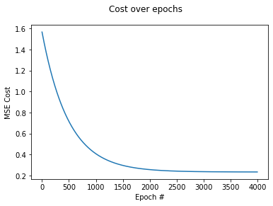
If we store the MSE after each training step (=epoch), we can plot how the cost changes over time. Notice that the step size will get smaller at each epoch, since the values in gradient are smaller. This will make the algorithm to ease-in towards the global minimum.

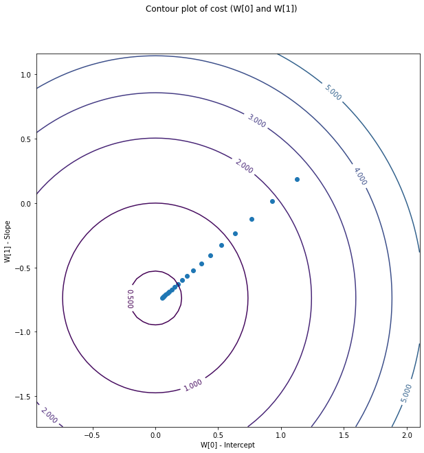
The data can also be plotted as a contour plot, where x and y axes represent the theta, which are the slope and the intercept when only one feature is present.

What we have just implemented is a (Vanilla) Gradient Descent that treats the whole dataset as a single batch. The weights are updated based on all samples in the datasets. When your dataset is massive, this is wasteful. There are multiple options to avoid this:

• Stochastic Gradient Descent (SGD). This would be easy to implement on our code, since we are already looping through the training samples one-by-one. Instead of appending the partial derivatives to a list, we would simply update the W on each sample. Note that this, too, would be slow on large dataset, since we would not be using our computers ability to perform rapid matrix operations.
• Mini-Batch SGD. This is a more common approach than either of the above: the vanilla or the one-sample solution. Mini-batch refers to a small selection of samples from our dataset. Imagine if we were to split our dataset into 10 equally-sized slices and perform a gradient step after each split. We should be able to still find the global minimum, right?
• Use some other optimization method. (S)GD and its variations aren't the only optimizers available, but they are wise-spread and common - especially in the field of deep learning. The LogisticRegressor in scikit learn calls these solvers and supports at least: newton-cg, lbfgs, liblinear, sag and saga. SciPy library's Optimize module has more options.

Regularization

Currently, our code is trying its best to minimize the output of the cost function.

# What we have been doing so far
minimize(cost)

Regularization will slow these steps down in order to avoid problems of overfitting. We haven't discussed this topic yet, so do not worry if the word "overfitting" is new to you. For now, believe that adding some regularization, also known as penalty, can be useful in certain scenarios.

# What we would want to do:
minimize(cost + regularization_term)

In scikit learn's SGDRegressor, the regularization is defined as: "The regularizer is a penalty added to the loss function that shrinks model parameters towards the zero vector using either the squared euclidean norm L2 or the absolute norm L1 or a combination of both (Elastic Net)".

Let's create a cost function with L2 penalty, also known as weight decay:

def l2_cost_function(y, y_hat, W, lambda_):
    errors = y_hat - y
    m = len(y)
    cost = 1/(2*m) *  sum(errors ** 2) + lambda_ * np.sum(W**2)
    return cost

The formula is:

$ cost = \frac{1}{2m}\sum(y-y_{hat})^2 + \lambda ||W||^2 $

Notice that both sides of the formula are similar (split by the plus sign.) The lambda symbol, λ, is the regularization rate that has been set by the user; it is a multiplier that scales how strong the regularization will be. Thus, the regularization term will be the sum of squared weights times the lambda. The lambda is usually a fairly small number, such as 0.01.

Before adding the regularization, the cost function didn't have any access the to weights (W). Now it does. By applying regularization, we can add penalty based on how large the weights are.

$ gradient = \frac{1}{m}X^T \cdot (y - y_{hat}) + \lambda W $

# Gradient with the regularization
gradient = (1/m) * X.T @ e + reg_rate * W

# Update the weights
W -= -learning_rate * gradient

NOTE! The W[0], the intercept, should not be regularized. We want to affect the slope; not the bias. Since we have included the bias into our X, we need to modify the code slightly.

# Same as above, but the intercept will not be regularized.
gradient = -(1/m) * X.T @ e
gradient[1:] += reg_rate * W[:1]

Let's perform a single step of gradient descent with various regularization rates:

# Use Boston dataset. All 13 features. Perform StandardScaling on X and y.
X = ss_x.fit_transform(boston.data)
y = ss_y.fit_transform(boston.target.reshape(-1, 1))

# Add the bias term
X = np.c_[ np.ones(len(y)), X]

# Randomize W
np.random.seed(42)
W = np.random.randn(X.shape[1], 1)

# Calculate the gradient. It will be vector with a lenght of 14.
gradient = (1/m) * X.T @ (y - (X @ W))

# Perform regularization
gradient[1:] = gradient[1:] + λ * W[1:]

The values we will be using are 0.0 (no regularization), 0.01 (a bit of regularization) and 0.1 (10x more regularization.) Note that the W has been randomized. Based on this W, the values in gradient vector are:

| W | Gradient (λ=0.0) | Gradient (λ = 0.01) | Gradient (λ= 0.1) | | ----- | ---------------- | ------------------- | ----------------- | | - 0.5 | -0.5 | -0.5 | -0.5 | | -0.14 | 0.27 | 0.27 | 0.26 | | 0.65 | -0.37 | -0.36 | -0.30 | | 1.52 | -0.19 | -0.17 | -0.04 | | … | … | … | … | | -1.91 | 1.24 | 1.22 | 1.04 |

As can be seen, the gradients have been shrunk towards 0 based on the how large the original W is. Remember that the step size will be computed using the learning rate.

step = -learning_rate * gradient
W -= step

Conclusion

This lesson might feel a bit overwhelming. Do not worry! This all will make sense when you learn how to plot learning curves and learn various useful concepts such as overfitting. What is important is to understand the intuition behind optimization and regularization.

• Optimization is finding the W that minimizes the cost function.
  • There are various optimization algorithms.
  • Learning rate (alpha, α) is the key parameter to tune.
• Regularization is any method that increases testing accuracy (usually at the cost of training cost).
  • Regression rate (lambda, λ) is the key parameter to tune.
    • Scikit learn calls this alpha, which can be confusing.
  • Common methods of applying regularization are L1 and L2.
    • L1 is also called as Lasso regularization.
    • L2 is also called as Ridge, weight decay or Tikhonov regularization.
    • ElasticNet mixes L1 and L2 using a weighted sum.

Usually, you don't have to write the code for optimization and regularization yourself, assuming you are using libraries such as scikit learn or TensorFlow. Different regularization methods work in different cases. For example, L1 regularization will shrink the least useful coefficient to zero, essentially performing feature selection. This can be useful when you have thousands of features. L2 can be considered as the 'default' regularization you will be using in most cases.

At this point, it is also fair to point out that all problems are not convex. Some problems, such as many faced by deep learning algorithms, have a bumpy cost landscape. Thus, there are local minima, which may not be the deepest potholes in the graph, but do look like one if you are a bee inside of it. Nevertheless, SGD is being used in deep neural networks: it may not find the global optimum for all of the weights, but it is usually performing well enough.

Before you continue to next lessons, compare the scikit learn documentation about Lasso regressor, Ridge regressor and ElasticNet regressor.